Bayesian Benefit Risk

Bayesian Benefit Risk

benefit(name, fun, weight)

risk(name, fun, weight)

br(...)

mcda(...)

Arguments

name

a string indicating the name of the benefit or risk.

fun

a utility function which maps a parameter value to a utility value.

weight

the weight of the benefit/risk.

...

calls to benefit(), risk(), and br_group() to define the utility functions and treatment groups.

Value

A named list with posterior summaries of utility for each group and the raw posterior utility scores.

Details

The br() function allows the user to define an arbitrary number of "benefits" and "risks". Each benefit/risk requires a utility function (fun) and a weight. The utility function maps the benefit/risk parameter to a utility score. The br_group() function supplies samples from the posterior distribution for each benefit risk for a specific group (e.g. treatment arm).

The br() function then calculates the posterior distribution of the overall utility for each group. The overall utility is a weighted sum of the utilities for each benefit/risk.

The mcda() function is the same as br(), but has extra checks to ensure that the total weight of all benefits and risks is 1, and that the utility functions produce values between 0 and 1 for all posterior samples.

Examples

set.seed(1132)
ilogit <- function(x) 1 / (1 + exp(-x))
out <- mcda(
  benefit("CV", function(x) ilogit(x), weight = .75),
  risk("DVT", function(x) ilogit(- .5 * x), weight = .25),
  br_group(
    label = "PBO",
    CV = rnorm(1e4, .1),
    DVT = rnorm(1e4, .1)
  ),
  br_group(
    label = "TRT",
    CV = rnorm(1e4, 2),
    DVT = rnorm(1e4, 1)
  )
)

out
#> # A tibble: 20,000 × 11
#>        CV CV_weight CV_uti…¹ CV_sc…²     DVT DVT_w…³ DVT_u…⁴ DVT_s…⁵ label  iter
#>     <dbl>     <dbl>    <dbl>   <dbl>   <dbl>   <dbl>   <dbl>   <dbl> <chr> <int>
#>  1  1.47       0.75    0.813   0.610  0.439     0.25   0.445  0.111  PBO       1
#>  2  0.239      0.75    0.559   0.420 -2.12      0.25   0.743  0.186  PBO       2
#>  3  0.969      0.75    0.725   0.544  0.974     0.25   0.381  0.0951 PBO       3
#>  4  0.655      0.75    0.658   0.494  0.0771    0.25   0.490  0.123  PBO       4
#>  5  1.51       0.75    0.819   0.615 -0.993     0.25   0.622  0.155  PBO       5
#>  6 -1.32       0.75    0.210   0.158 -0.874     0.25   0.607  0.152  PBO       6
#>  7  0.395      0.75    0.598   0.448  1.03      0.25   0.375  0.0936 PBO       7
#>  8 -1.43       0.75    0.193   0.145 -0.903     0.25   0.611  0.153  PBO       8
#>  9  0.180      0.75    0.545   0.409 -0.685     0.25   0.585  0.146  PBO       9
#> 10 -0.960      0.75    0.277   0.208 -1.50      0.25   0.679  0.170  PBO      10
#> # … with 19,990 more rows, 1 more variable: total <dbl>, and abbreviated
#> #   variable names ¹​CV_utility, ²​CV_score, ³​DVT_weight, ⁴​DVT_utility,
#> #   ⁵​DVT_score

summary(out, probs = c(.025, .5, .975))
#> $summary
#> # A tibble: 2 × 5
#>   label  mean `2.50%` `50.00%` `97.50%`
#>   <chr> <dbl>   <dbl>    <dbl>    <dbl>
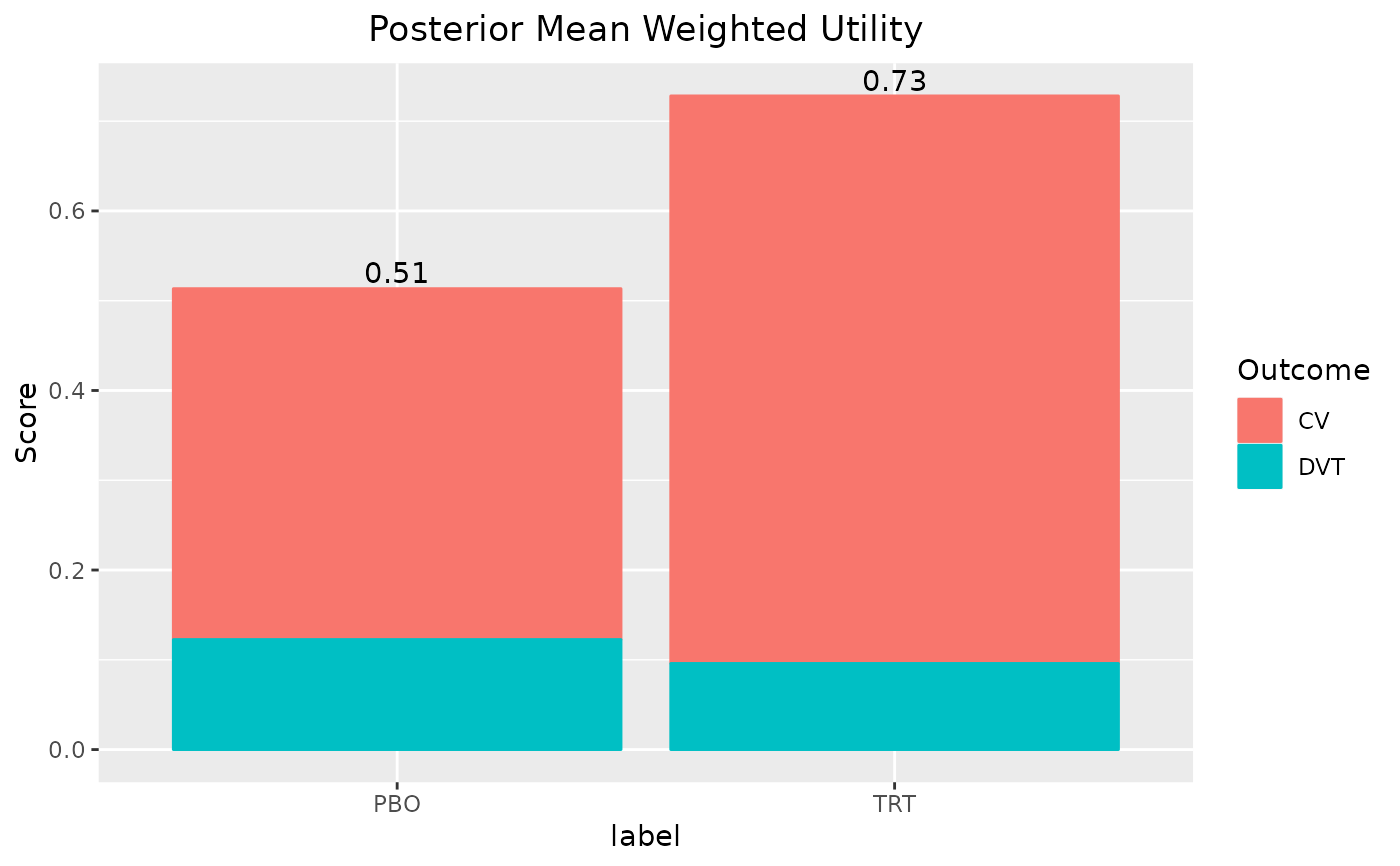
#> 1 PBO   0.513   0.221    0.518    0.794
#> 2 TRT   0.728   0.472    0.752    0.857
#> 
#> $scores
#> # A tibble: 20,000 × 11
#>        CV CV_weight CV_uti…¹ CV_sc…²     DVT DVT_w…³ DVT_u…⁴ DVT_s…⁵ label  iter
#>     <dbl>     <dbl>    <dbl>   <dbl>   <dbl>   <dbl>   <dbl>   <dbl> <chr> <int>
#>  1  1.47       0.75    0.813   0.610  0.439     0.25   0.445  0.111  PBO       1
#>  2  0.239      0.75    0.559   0.420 -2.12      0.25   0.743  0.186  PBO       2
#>  3  0.969      0.75    0.725   0.544  0.974     0.25   0.381  0.0951 PBO       3
#>  4  0.655      0.75    0.658   0.494  0.0771    0.25   0.490  0.123  PBO       4
#>  5  1.51       0.75    0.819   0.615 -0.993     0.25   0.622  0.155  PBO       5
#>  6 -1.32       0.75    0.210   0.158 -0.874     0.25   0.607  0.152  PBO       6
#>  7  0.395      0.75    0.598   0.448  1.03      0.25   0.375  0.0936 PBO       7
#>  8 -1.43       0.75    0.193   0.145 -0.903     0.25   0.611  0.153  PBO       8
#>  9  0.180      0.75    0.545   0.409 -0.685     0.25   0.585  0.146  PBO       9
#> 10 -0.960      0.75    0.277   0.208 -1.50      0.25   0.679  0.170  PBO      10
#> # … with 19,990 more rows, 1 more variable: total <dbl>, and abbreviated
#> #   variable names ¹​CV_utility, ²​CV_score, ³​DVT_weight, ⁴​DVT_utility,
#> #   ⁵​DVT_score
#> 
summary(out, reference = "PBO")
#> $summary
#> # A tibble: 1 × 5
#>   label  mean `2.50%` `97.50%` reference
#>   <chr> <dbl>   <dbl>    <dbl> <chr>    
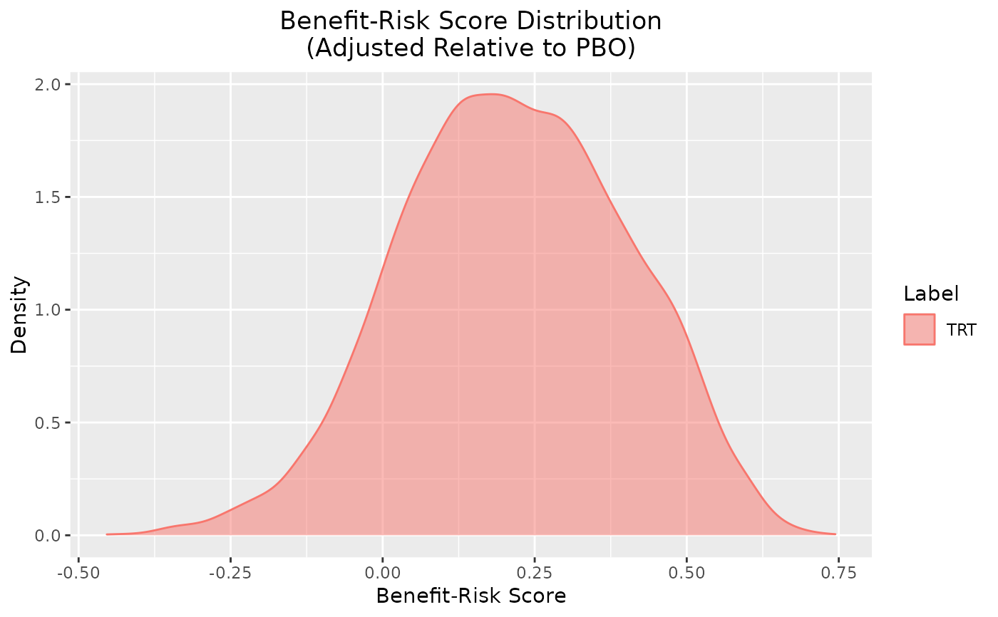
#> 1 TRT   0.215  -0.150    0.555 PBO      
#> 
#> $scores
#> # A tibble: 10,000 × 12
#>       CV CV_weight CV_utility CV_sc…¹    DVT DVT_w…² DVT_u…³ DVT_s…⁴ label  iter
#>    <dbl>     <dbl>      <dbl>   <dbl>  <dbl>   <dbl>   <dbl>   <dbl> <chr> <int>
#>  1 1.01       0.75      0.733   0.550 0.381     0.25   0.453  0.113  TRT       1
#>  2 1.66       0.75      0.841   0.631 1.84      0.25   0.285  0.0713 TRT       2
#>  3 0.473      0.75      0.616   0.462 0.403     0.25   0.450  0.112  TRT       3
#>  4 2.59       0.75      0.930   0.698 0.0774    0.25   0.490  0.123  TRT       4
#>  5 2.39       0.75      0.916   0.687 2.47      0.25   0.225  0.0563 TRT       5
#>  6 2.43       0.75      0.919   0.689 1.08      0.25   0.368  0.0920 TRT       6
#>  7 1.58       0.75      0.828   0.621 2.02      0.25   0.267  0.0667 TRT       7
#>  8 3.10       0.75      0.957   0.718 1.04      0.25   0.373  0.0932 TRT       8
#>  9 3.48       0.75      0.970   0.728 0.644     0.25   0.420  0.105  TRT       9
#> 10 1.10       0.75      0.750   0.563 0.586     0.25   0.427  0.107  TRT      10
#> # … with 9,990 more rows, 2 more variables: total <dbl>, reference <chr>, and
#> #   abbreviated variable names ¹​CV_score, ²​DVT_weight, ³​DVT_utility, ⁴​DVT_score
#> 

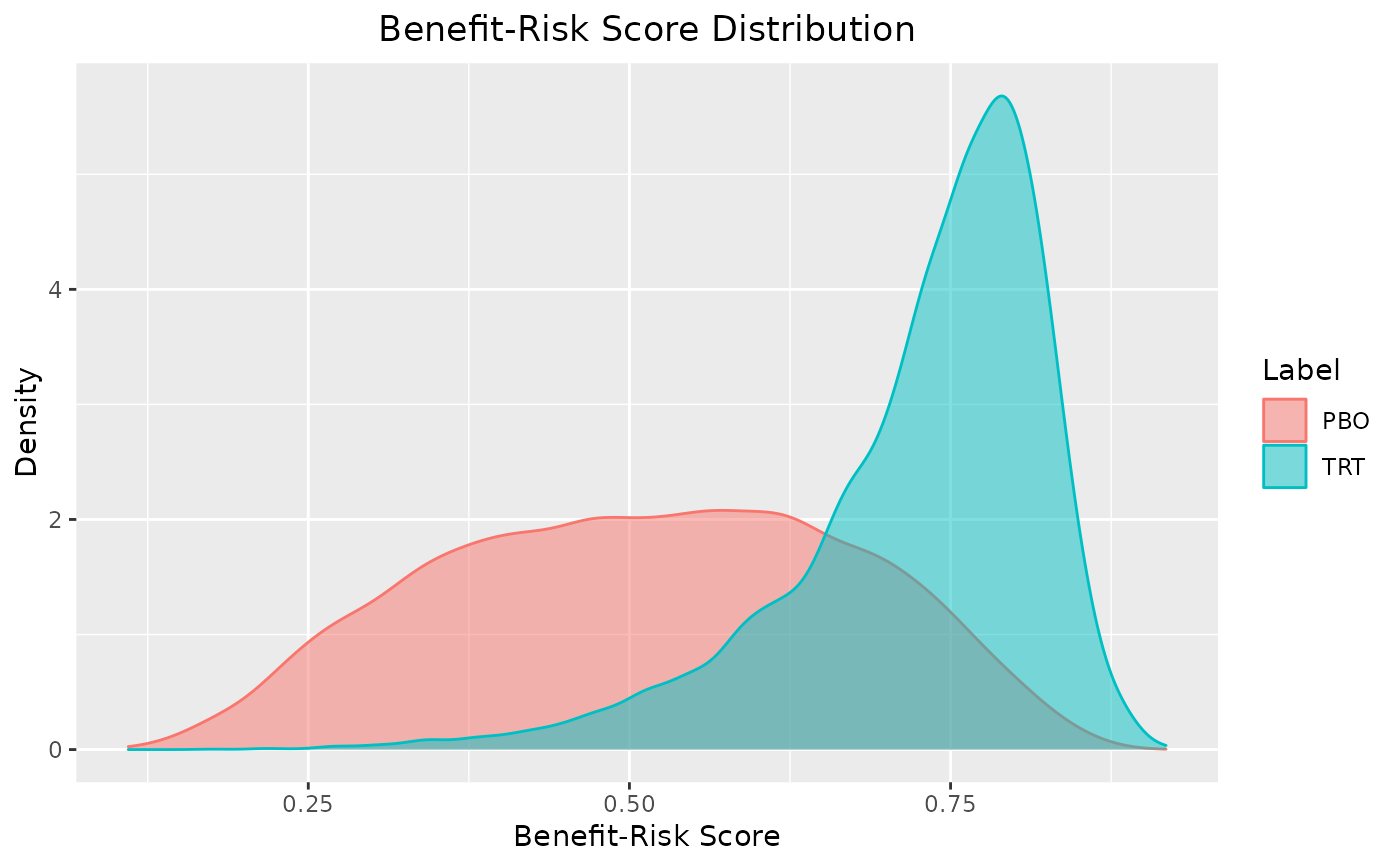
plot(out)

plot(out, reference = "PBO")


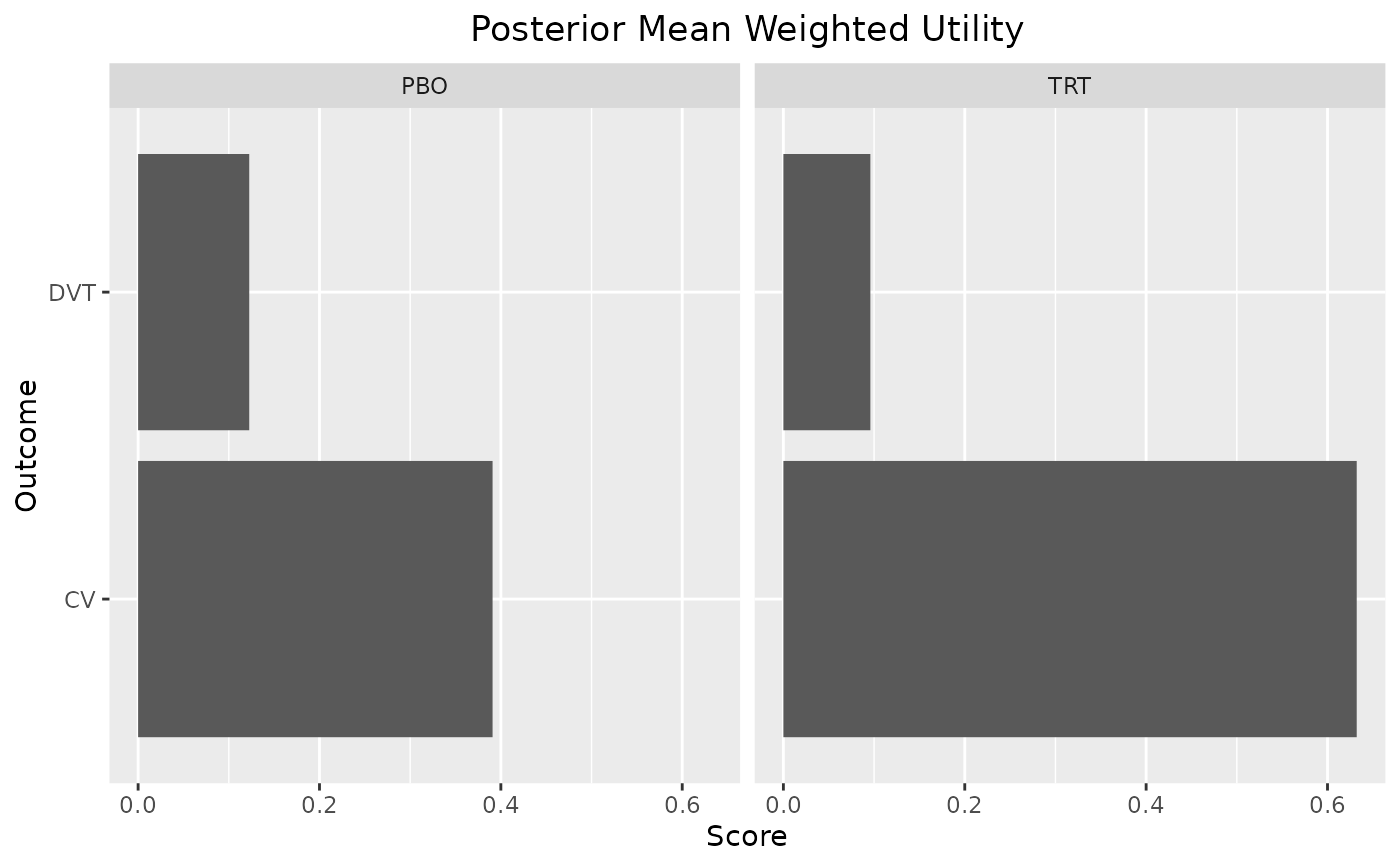
plot_utility(out)

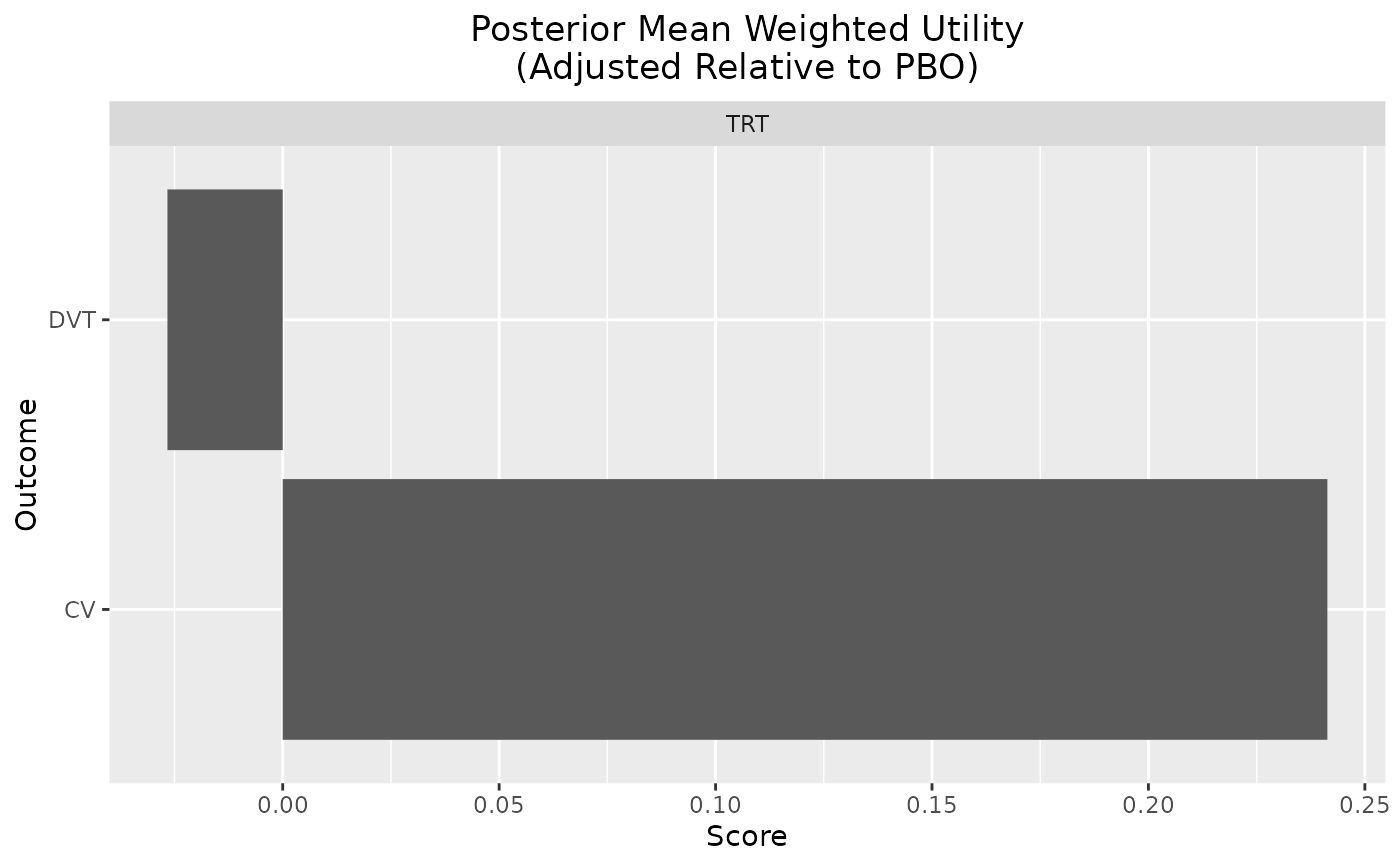
plot_utility(out, reference = "PBO")

plot_utility(out, stacked = TRUE)