Compare Posterior Fits
plot_comparison(..., doses, times, probs, data, n_smooth, width)

# Default S3 method
plot_comparison(
  ...,
  doses = attr(list(...)[[1]], "doses"),
  times = NULL,
  probs = c(0.025, 0.975),
  data = NULL,
  n_smooth = 50,
  width = bar_width(doses)
)

# S3 method for class 'dreamer_bma'
plot_comparison(
  ...,
  doses = x$doses,
  times = NULL,
  probs = c(0.025, 0.975),
  data = NULL,
  n_smooth = 50,
  width = bar_width(doses)
)
Arguments
- ...
dreamer_mcmcobjects to be used for plotting.- doses
a vector of doses at which to plot the dose response curve.
- times
the times at which to do the comparison.
- probs
quantiles of the posterior to be calculated.
- data
a dataframe with column names of "dose" and "response" for individual patient data. Optional columns "n" and "sample_var" can be specified if aggregate data is supplied, but it is recommended that patient-level data be supplied where possible for continuous models, as the posterior weights differ if aggregated data is used. For aggregated continuous data, "response" should be the average of "n" subjects with a sample variance of "sample_var". For aggregated binary data, "response" should be the number of successes, "n" should be the total number of subjects (the "sample_var" column is irrelevant in binary cases and is ignored).
- n_smooth
the number of points to calculate the smooth dose response interpolation. Must be sufficiently high to accurately depict the dose response curve.
- width
the width of the error bars.
Value
a ggplot object.
Details
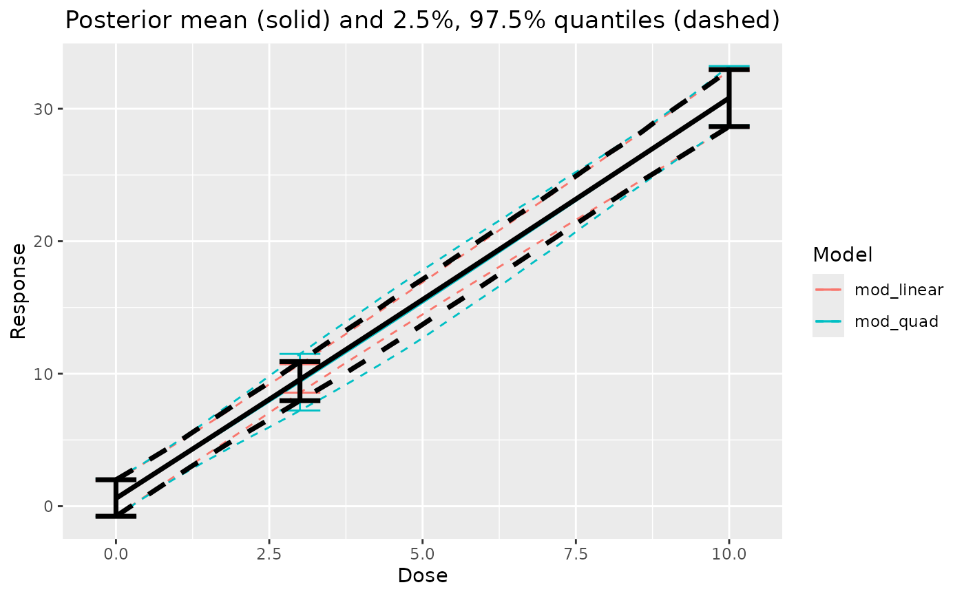
If a Bayesian model averaging object is supplied first, all individual fits and the Bayesian model averaging fit will be plotted, with the model averaging fit in black (other model colors specified in the legend). Otherwise, named arguments must be supplied for each model, and only the models provided will be plotted.
Examples
set.seed(888)
data <- dreamer_data_linear(
n_cohorts = c(20, 20, 20),
dose = c(0, 3, 10),
b1 = 1,
b2 = 3,
sigma = 5
)
# Bayesian model averaging
output <- dreamer_mcmc(
data = data,
n_adapt = 1e3,
n_burn = 1e3,
n_iter = 1e3,
n_chains = 2,
silent = FALSE,
mod_linear = model_linear(
mu_b1 = 0,
sigma_b1 = 1,
mu_b2 = 0,
sigma_b2 = 1,
shape = 1,
rate = .001,
w_prior = 1 / 2
),
mod_quad = model_quad(
mu_b1 = 0,
sigma_b1 = 1,
mu_b2 = 0,
sigma_b2 = 1,
mu_b3 = 0,
sigma_b3 = 1,
shape = 1,
rate = .001,
w_prior = 1 / 2
)
)
#> mod_linear
#> start : 2024-12-19 14:43:27.252
#> Compiling model graph
#> Resolving undeclared variables
#> Allocating nodes
#> Graph information:
#> Observed stochastic nodes: 6
#> Unobserved stochastic nodes: 3
#> Total graph size: 50
#>
#> Initializing model
#>
#> finish: 2024-12-19 14:43:27.270
#> total : 0.02 secs
#> mod_quad
#> start : 2024-12-19 14:43:27.270
#> Compiling model graph
#> Resolving undeclared variables
#> Allocating nodes
#> Graph information:
#> Observed stochastic nodes: 6
#> Unobserved stochastic nodes: 4
#> Total graph size: 59
#>
#> Initializing model
#>
#> finish: 2024-12-19 14:43:27.289
#> total : 0.02 secs
plot_comparison(output)
 # compare individual models
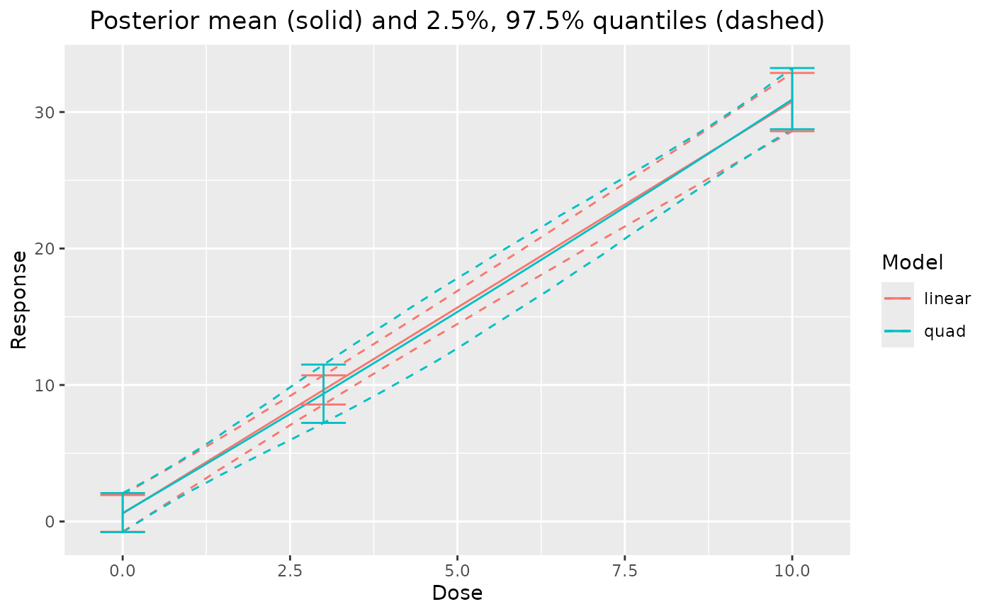
plot_comparison(linear = output$mod_linear, quad = output$mod_quad)
# compare individual models
plot_comparison(linear = output$mod_linear, quad = output$mod_quad)